Rai's ML mistakes, part 3 of ∞

Posted on 2021-10-18

Previous parts:

Next step: half-cheetah, TD3, continuous actions

I’m not doing all that great emotionally, but I’m trying to keep learning RL, even if slowly. I made Cartpole and Lunar Landing environments work. Both of them have discrete actions. The next environment I went to try to learn was the Half Cheetah.

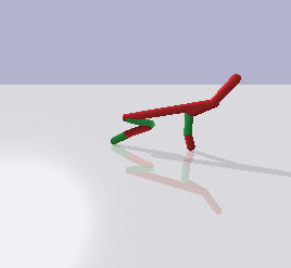
In this environment, you control a simple robot and are trying to teach it to run. You control it with continuous signals. I’m not sure what exactly they mean, probably something like force applied to joints. Continuous actions mean you need to use slightly different algorithms. I went to learn TD3 (twin delayed deep deterministic actor-critic), based on OpenAI’s treatment in Spinning Up in Deep RL. It was published in a 2018 paper called Addressing Function Approximation Error in Actor-Critic Methods.

Sidenote: depending on MuJoCo sucks

The vanilla half-cheetah environment is written with MuJoCo. MuJoCo is a commercial physics simulator used for a lot of robotics environments like this. You need a license to run it. As of now (October 18, 2021), there is a free license available for everyone to run MuJoCo until the end of this month. But in general, closed-source dependencies for open research suck.

There’s this open-source physics engine called Bullet. I’ve played with it a bit in middle-high school when I was trying to write some 3D stuff. Turns out they have since made Python bindings, and implemented a bunch of OpenAI Gym environments. So you can now run lots of environments without MuJoCo :)

To use the PyBullet environments, install the pybullet Python package and import pybullet_envs. The PyBullet repo has the list of implemented environments.

Sidenote 2: Actually MuJoCo is now open-source

So, later on the same day I wrote this post, turns out DeepMind bought MuJoCo and made it open-source and free (at https://mujoco.org/). Good stuff :)

TD3 description

Q learning

To describe TD3 briefly, it’s similar to Q learning.

In Q learning, you’re learning a function $\hat{\mathrm{Q}}_\theta(s,a)$, and a policy $\pi$. You update $\theta$ to make $\hat{\mathrm{Q}}_\theta(s,a)$ match closer to the actual Q function for the policy $\pi$, and you also update the policy $\pi$ to gradually improve. You can do this exactly if you have a small enough environment to hold all this in memory. The procedure you use to make $\hat{\mathrm{Q}}_\theta$ approximate $\mathrm{Q}_\pi$ is basically SARSA: you minimize the squared error between $\hat{\mathrm{Q}}_\theta(s,a)$ and an estimator that converges to center on the actual $\mathrm{Q}_\pi(s,a)$. In the finite case, that Q learning estimator for a transition $s \xrightarrow{a} (r, s’)$ is $r + \gamma \max_{a’} \hat{\mathrm{Q}}_\theta(s’,a’)$. In vanilla Q learning, the followed policy is $\mathrm{greedy}(\hat{\mathrm{Q}})$, which is what that maximum does.

But when you’re in a continuous action space, you can’t just $\arg\max$ over all possible actions.

DDPG

Enter DDPG (Deep Deterministic Policy Gradient), in which you maintain 2 networks: the critic $\hat{\mathrm{Q}}_\theta(s,a)$ which approximates the Q value of the current policy, and the actor - a deterministic policy $\pi_\varphi: \mathcal{S} \rightarrow \mathcal{A}$, which you improve based on the critic’s estimations.

Run the agent with your current policy in a replay buffer, plus with some exploration (like a bit of Gaussian noise added to actions). Draw a batch from the replay buffer, and do an optimization step on the critic to minimize its Bellman error: $$\arg\min_\theta \sum_{(s,a,r,s') \in \mathrm{batch}} \left[\hat{\mathrm{Q}}_\theta(s,a) - (r + \gamma \hat{\mathrm{Q}}_\theta(s', \pi_\varphi(s')))\right]^2 $$ Then update the actor to choose actions that get better Q values on the same batch: $$\arg\max_\varphi \sum_{(s,a) \in \mathrm{batch}} \hat{\mathrm{Q}}_\theta(s,\pi_\varphi(s))$$ The batch has to be drawn randomly. This is important, because if you draw a bunch of states that immediately follow each other, their predictions will end up pulling each other to explode towards infinity.

To prevent similar feedback cycles between the actor and critic, you keep 2 copies of each: the optimized one and the target one. They start out as exact copies. When computing the Bellman targets for the critic, instead of using the optimized actor and critic, use the target ones: $$\arg\min_\theta \sum_{(s,a,r,s') \in \mathrm{batch}} \left[\hat{\mathrm{Q}}_{\theta_\text{opt}}(s,a) - (r + \gamma \hat{\mathrm{Q}}_{\theta_\text{targ}}(s', \pi_{\varphi_\text{targ}}(s')))\right]^2 $$ And slowly Polyak-average the target networks towards the optimized one (with (\approx 0.05)): $$ \begin{align*} \theta_\text{targ} & \gets \varrho \cdot \theta_\text{opt} + (1-\varrho) \cdot \theta_\text{targ} \\ \varphi_\text{targ} & \gets \varrho \cdot \varphi_\text{opt} + (1-\varrho) \cdot \varphi_\text{targ} \end{align*} $$ By the way, I made up this a shorthand notation for this operation “update x towards y with update size (\alpha)”: $$\require{extpfeil} \theta_\text{targ} \xmapsto{\varrho} \theta_\text{opt}, \varphi_\text{targ} \xmapsto{\varrho} \varphi_\text{opt} $$

TD3

Twin Delayed Deep Deterministic Policy Gradient was introduced in a paper called Addressing Function Approximation Error in Actor-Critic Methods. Note the “function approximation error” part. This talks about the error inherent in how $\hat{\mathrm{Q}}_\theta$ approximates the real $\mathrm{Q}_\pi$. In particular, if in a state $s$, the critic overestimates the Q value for some action $a$, the actor’s optimization step will be incentivized to exploit that overestimation. But that doesn’t mean it’ll actually get a better result.

TD3 adds 3 steps to address this:

Target policy smoothing: in the Bellman update, instead of expecting to follow $\pi_{\varphi_\text{targ}}$ exactly, add a bit of Gaussian noise to the chosen action. That way the policy can’t try to hit a small peak of overestimation by the critic.
Twin critics: train 2 critics, both to minimize the Bellman error. Optimize the policy to maximize one of them. Instead of setting critics’ targets based on one critic, choose the target based on the lesser of their two predictions. If you train 2 networks, they’re unlikely to overestimate the real Q function in the same place. $$\arg\min_\theta \sum_{i \in {1, 2}} \sum_{(s,a,r,s') \in \mathrm{batch}} \left[\hat{\mathrm{Q}}_{\theta_{i, \text{opt}}}(s,a) - (r + \gamma \min_{j\in {1, 2}}\hat{\mathrm{Q}}_{\theta_{j, \text{targ}}}(s', \pi_{\varphi_\text{targ}}(s')))\right]^2 $$
Delayed policy updates: update the policy just once per 2 batches (i.e., 2x slower than the critics).

Rai’s ML mistake #5: Multiplication? What multiplication?

The following happened over the course of ~6 weeks, as I gathered a few hours at a time of energy, will, etc. to work on this.

So, I go and implement my algorithm and run it. On my first try, I implement it wrong because I misremember how to implement it. I go back to Spinning Up in Deep RL, smack myself on the forehead, and go fix it. Run it again.

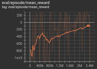
It’s learning something. The average reward is going up. But slowly.

Then, over the next ~4 weeks, whenever I have some time, I try to bang my head against the keyboard some more. Tweak all the hyperparameters. Look up the hyperparameters they use in rl-baselines3-zoo. No dice. Repeat for a while, for all hyperparameters - critic learning rate, actor learning rate, actor delay, replay buffer size, batch size, Polyak rate, discount rate, initial random action steps. Rewrite the code twice-thrice. Still the same issue. Keep it training for several days. Does not help. Repeat a few times.

Thanks God there’s a reference implementation

I wanted to implement this algorithm on my own, because I want to grok it. But I got to the end of my wits here, and started thinking: “hell, can this algorithm even solve this environment”? The paper had graphs and results with the half-cheetah. But that was the MuJoCo half-cheetah. Maybe the PyBullet half-cheetah had a different reward scale and this was actually as good as it went?

Unlikely. All my half-cheetah did in evaluation was stand upright without moving. Maybe sometimes kinda jump once.

But yeah. Let’s run the reference implementation and see what it does. I start it for a few minutes, and…

...
Total T: 109000 Episode Num: 109 Episode T: 1000 Reward: 938.893
Total T: 110000 Episode Num: 110 Episode T: 1000 Reward: 987.304
---------------------------------------
Evaluation over 10 episodes: 963.088
---------------------------------------

God dammit. I was getting maybe, on a lucky episode, like 300 at most, and that was after millions of training steps…

Does it just not work because of Tensorflow?!

Okay, so I have code A which does not work (my code), and code B which does (reference implementation). I know what to do here. Align code A and code B together so that they’re similar, and then scour the diff line by line. Somewhere in there there’s my bug.

I refactor my code, rename variables, etc., until the diff is small.

Now the only diff I see is basically me using Tensorflow and the reference implementation using PyTorch. Stuff like this:

2,3c3,7
< import tensorflow as tf
< from tensorflow.keras import layers as tfkl
---
> import torch
> import torch.nn as nn
> import torch.nn.functional as F
136,137c123,124
<         state = tf.expand_dims(state, axis=0)
<         return tf.squeeze(self.actor(state), axis=0).numpy()
---
>         state = torch.FloatTensor(state.reshape(1, -1)).to(device)
>         return self.actor(state).cpu().data.numpy().flatten()

And yet, my code doesn’t work, and their code does.

I bang my head against this for maybe 2 more days. So, where can the differences be?

Maybe different action scaling. I align action scaling like they do. Instead of “sigmoid, then rescale from 0 to 1 into action_space.low to action_space.high”, I do their “tanh, then multiply by action_space.high”. Those should be basically the same thing, but I do it anyway just to be safe. Still doesn’t work.

Maybe different initialization. Unlikely, but possible. Their code uses Torch’s Linear. It initializes weights and biases both randomly from $\text{Uniform}([\pm \sqrt{\frac{1}{\text{input size}} }])$. I use TensorFlow/Keras’s Dense. It uses Xavier uniform initialization (aka Glorot initialization, named … after someone named Xavier Glorot) by default, which draws from $\text{Uniform}([\pm \sqrt{\frac{6}{\text{input size} + \text{output size} } }])$. And TensorFlow initializes biases to zero. Okay. I rewrite the TensorFlow initialization to do the same thing as Torch. Still the same. God dammit.

Does the ADAM optimizer in TensorFlow and PyTorch work differently? … Maybe. I’m gonna shelve the idea of stepping through it for later.

Copy the whole goddamn setup

I decide that I’ll copy even more of their code. Okay, this is unlikely, but what if there’s something wrong with how I initialize the environment or something? I copy their main.py, switch it to TensorFlow, and use their utils.py.

And now it works, and I scream.

It’s the utils.py that did it. That file in their repo implements the replay buffer. I didn’t pore over my implementation in detail, because … hey, it’s the simplest part. How would I mess up a replay buffer?

Their replay buffer exists in RAM, and has NumPy arrays. It uses NumPy’s randomness. I use TensorFlow variables and TensorFlow’s tf.random.Generator.

After some work, I find the culprit lines.

Here’s how my code stores the replay buffer’s rewards and “is this the final state” flag:

class ReplayBuffer:
    def __init__(self, state_dim, action_dim, max_size=int(1e6)):
	# ... snip ...
        self.reward = tf.Variable(tf.zeros((max_size, )), dtype=tf.float32)
        self.not_done = tf.Variable(tf.zeros((max_size, ), dtype=tf.float32),
                                    dtype=tf.float32)

And this is how they do it:

class ReplayBuffer(object):
    def __init__(self, state_dim, action_dim, max_size=int(1e6)):
	# ... snip ...
        self.reward = np.zeros((max_size, 1))
        self.not_done = np.zeros((max_size, 1))

What’s the difference? I have a vector, a 1-dimensional tensor. They have a 2-dimensional tensor, with second dimension 1.

And of course it’s goddamn tensor shapes.

On its own, it doesn’t matter whether I have the replay buffer shaped like I had it, or like they did.

What matters is what happens when I combine it with this code which computes the target Q values:

# Select action according to policy and add clipped noise
noise = tf.random.normal(shape=action.shape) * self.policy_noise
noise = tf.clip_by_value(noise, -self.noise_clip, self.noise_clip)

next_action = (self.actor_target(next_state) + noise)
next_action = tf.clip_by_value(next_action, -self.max_action,
			       self.max_action)

# Compute the target Q value
target_Q1, target_Q2 = self.critic_target((next_state, next_action))
target_Q = tf.math.minimum(target_Q1, target_Q2)
target_Q = reward + not_done * self.discount * target_Q

TD3 maintains 2 critics. critic_target is a Keras model, which contains two stacks of feed-forward layers. At the end, they have a q_value = tf.keras.layers.Dense(1, ...), and then the whole model returns the tuple (q1_value, q2_value).

With that in mind, what’s the shape of target_Q1?

No, it’s not (batch size). It’s (batch size,1). Because of course there’s the last dimension of size 1 - if your model has more than 1 output node, you need to stack them.

What’s the shape of not_done?

With my replay buffer, it was (batch size). One scalar per experience in batch, right? With the reference implementation’s replay buffer, it was (batch size,1).

Consider the line target_Q = reward + not_done * self.discount * target_Q, where target_Q has shape (batch size,1) and, as established for my code, not_done has shape (batch size). What’s the shape of the computed expression?

If you answered (batch size,batch size), I guess you win. And that was not intended. I wanted it to be (batch size) - one target Q value for one replay experience in batch.

What happens next with this target_Q?

@tf.function
def _mse(x, y):
    return tf.reduce_mean(tf.math.squared_difference(x, y))

with tf.GradientTape() as tape:
    # Get current Q estimates
    current_Q1, current_Q2 = self.critic((state, action))

    # Compute critic loss
    critic_loss = (_mse(current_Q1, target_Q) +
		   _mse(current_Q2, target_Q))

# Optimize the critic
self.critic_optimizer.minimize(
    critic_loss, tape=tape, var_list=self.critic.trainable_variables)

… Great. current_Q1 / current_Q2 have shapes (batch size,1), which is compatible with (batch size,batch size). So they get auto-broadcast… and reduce_mean gladly reduces the matrix of squared errors to a scalar mean. Awesome. Thank you. I’m so glad Autobroadcast Man and Default Options Girl arrived and saved the day.

Learnings

So what did I learn today?

It’s always, always, ALWAYS those goddamn tensor shapes.

Put tf.debugging.assert_shapes f***ing everywhere.

And probably write unit tests, too. I probably won’t be bothered to do that anyway because writing unit tests for code that has complex optimizers and neural nets is annoying.

And maybe I should be using operators that don’t auto-broadcast, or something that doesn’t allow me to mistakenly vector-vector-to-matrix multiply when I mean to vector-vector-elementwise multiply.

I’m not done being annoyed and sour about this but I’m done ranting about it here. Ciao, see you next time I kill a few weeks on another mistake this stupid. This is the point of all those “Rai’s ML mistakes” posts. I write these algorithms so I can grok them, and I headsmash the keyboard this way because I hope now I’ll remember with a bit more clarity and immediacy: “It’s always the goddamn tensor shapes”.

My fixed code is on my GitLab, and here’s the obligatory scoot-scoot:

A half-cheetah doing the scoot-scoot after 216 episodes of training.

Update: MuJoCo half-cheetah

So, since MuJoCo is now open-source, I tried it and got the MuJoCo environment HalfCheetah-v2 also working. Nice :)

Trained MuJoCo half-cheetah. Episode reward is 5330.